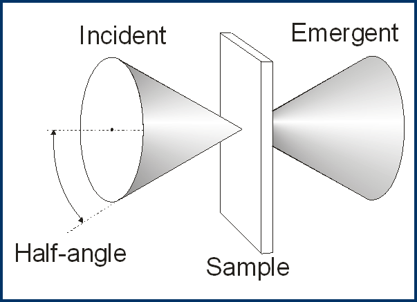
| When a sample is inserted at the focus of a convergent beam (at the focal plane), then biconical transmittance should be calculated:
\[T_b=\frac{total \; flux\; in \;output \;beam}{total\; flux\; in\; input \;beam}\]. The biconical transmittance \(T_b\) can be calculated as follows: \[ T_b=\frac{\int_{\varphi=0}^{2\pi}\int_{\xi=0}^{\xi_max} I(\xi,\varphi)T(\xi,\varphi)\sin\xi d\xi d\varphi}{\int_{\varphi=0}^{2\pi}\int_{\xi=0}^{\xi_max} I(\xi,\varphi)\sin\xi d\xi d\varphi}, \] where the angles \(\xi\) and \(\varphi\) are polar and azimuthal angles defined in the spherical coordinate system. The \(\xi_{\max}\) is the maximum semi-angle of the convergent cone. |
 |
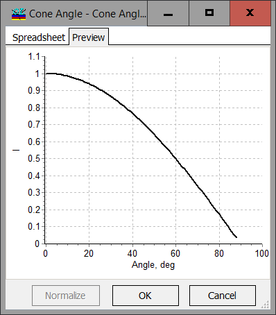
| In the case of Lambertian source \(I(\xi,\varphi)=I_0\cos\xi\) and equations can be simplified:
\[ T_b=(\pi \sin^2\xi_{\max})_{\varphi=0}^{-1}\int_{\varphi=0}^{2\pi}\int_{\xi=0}^{\xi_{\max}}T(\xi,\varphi)\sin\xi\cos\xi d\xi d\varphi.\] In the case when the principal ray of the cone is perpendicular to the multilayer sample the formula can be further simplified: \[T_b=2(\sin\xi_{\max})^{-2}\int_{\xi=0}^{\xi_{\max}} T(\xi)\sin\xi\cos\xi d\xi\] |
Cone Angle database of OptiLayer allows you to create cone angles averaging specifications. When Cone Angle is loaded to the memory, all computations of Transmittance, Reflectance, Back Reflectance, and Absorptance take into account cone angle averaging. All synthesis procedures also will take into account cone averaging. The only exclusion from this rule is a target with UDT characteristics.
If a design of a coating with different Cone Angle specifications are required, it can be performed with the help of Multi-Environment option of OptiLayer. |
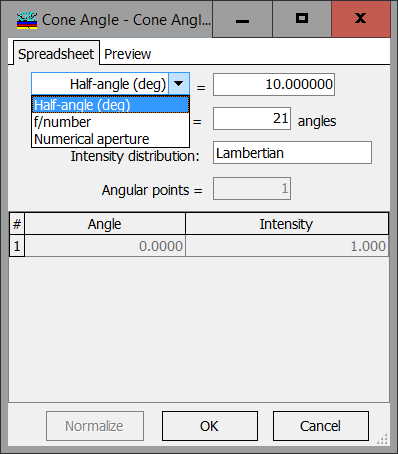
| Cone can be specified with Half-angle (in degrees), f/number or Numerical aperture. Computations are performed on angular grid, with growing number of points the accuracy is improving, but computational time is growing proportionally. OptiLayer uses high-precision sophisticated integration procedures, so for most cases 10-20 points are quite sufficient.
|
Type of distribution can be Uniform Intensity, Lambertian, or User-Defined. In the last case Cone Angle Editor allows to specify the number of Angular points for Cone Angle Intensity distribution and the spreadsheet itself. The number of angular points should not coincide with Cone averaging grid parameter. OptiLayer will perform all necessary interpolation procedures automatically.
|
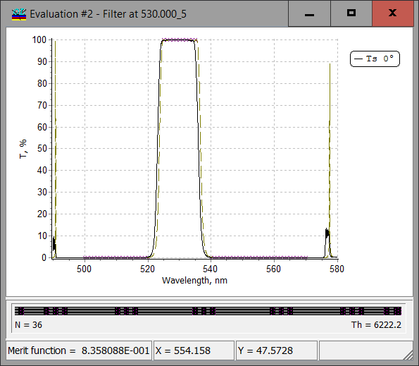
| Example: Comparison of a narrow bandpass filter without taking into account cone angle (solid curve) and with taking into account cone angle (dashed curve)
|
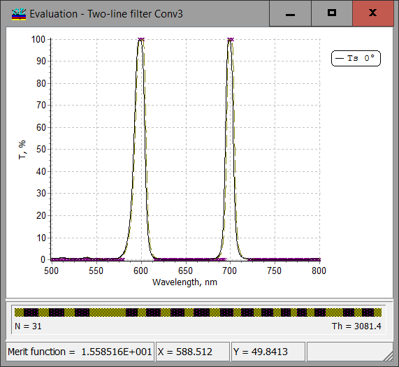
Example: Comparison of a two-line filter without taking into account cone angle (solid curve) and with taking into account cone angle (dashed curve)
|
OptiLayer provides user-friendly interface and a variety of examples allowing even a beginner to effectively start to design and characterize optical coatings. Read more…
Comprehensive manual in PDF format and e-mail support help you at each step of your work with OptiLayer.
If you are already an experienced user, OptiLayer gives your almost unlimited opportunities in solving all problems arising in design-production chain. Visit our publications page.
Look our video examples at YouTube
OptiLayer videos are available here:
Overview of Design/Analysis options of OptiLayer and overview of Characterization/Reverse Engineering options.
The videos were presented at the joint Agilent/OptiLayer webinar.