|
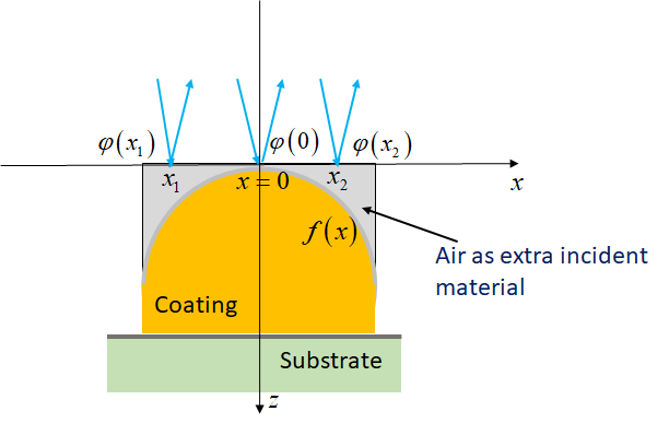
New option Wavefront/Taper analysis is implemented. The new option allows you to estimate the influence of inhomogeneities of the deposition on the spectral characteristics and on the wavefront of the reflected/transmitted wave. The option is available at Analysis –>More–>Wavefront/Taper Phase computations include total path of the beam including extra space in the incident medium due to changed total thickness of the coating at different positions (Fig. 1). Example:
|
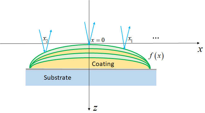
Fig. 1. Schematic of the coating with thickness non-uniformity. To calculate the effect of a lack of uniformity on the wavefront, an extra incident material (gray region) is added to the front surface of the coating, so that the reference surface for phase calculations is completely free from non-uniformity. |
|
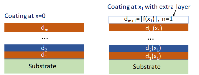
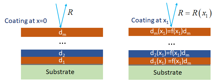
Fig. 2. Schematic of the multilayer at the central position (left) and the multilayer at the position x1 (right). |
Phase at different positions can be calculated as phase of the amplitude reflection coefficient in the following way: \[ \varphi (x=0):\;\;\; r(d_1,…,d_m)\] \[ \varphi (x=x_1):\;\;\; r(d_1(x_1),…,d_m(x_m))\] Wavefront can be calculated and plotted vs. the wavelength or relative coordinate \(x\) : \[ \delta R(\lambda)=\frac{\varphi(\lambda)}{2\pi} \] \[ \delta R(x)=\frac{\varphi(x)}{2\pi} \] |
|
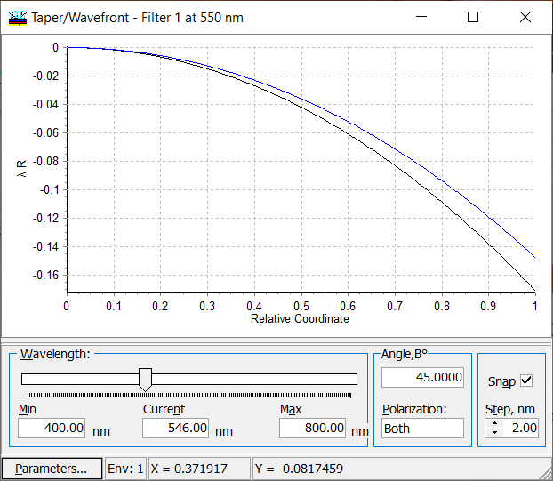
Fig. 3. Dependence of the reflected wavefront vs. relative coordinate calculated for parabolic taper interpolation specified in Fig. 3. The wavelength can be varied using the slider on the bottom of the window. |
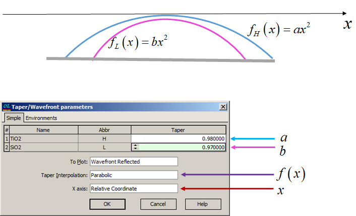
In the window Taper/Wavefron parameters available by pressing Parameters button, you can choose between Simple taper function \(f(x)\) and more complicated taper dependence specified in Environments tab. Example. \(f(x)\) are parabolic functions defined through taper coefficients \(a\) and \(b\) for high- and low-index materials, respectively (Fig. 4).
Fig. 4. Schematic of the parabolic non-uniformity and correspondence window in OptiLayer. |
|
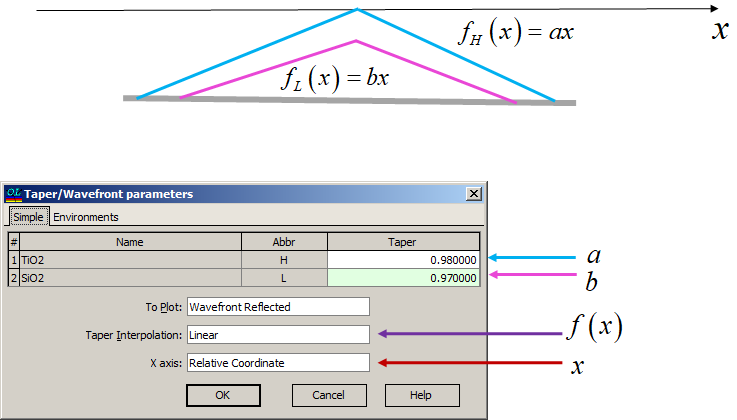
Example. \(f(x)\) can be specified as a linear function through \(a\) and \(b\) for high- and low-index materials, respectively (Fig. 5).
Fig. 5. Schematic of the parabolic non-uniformity and correspondence window in OptiLayer. |
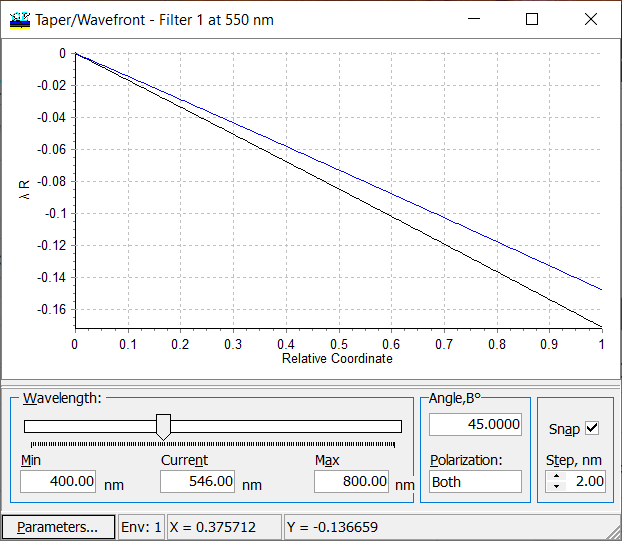
Fig. 6. Dependence of the reflected wavefront vs. relative coordinate calculated for linear taper interpolation specified in Fig. 5. The wavelength can be varied using the slider on the bottom of the window. |
|
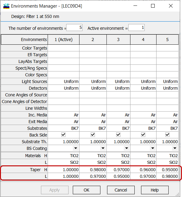
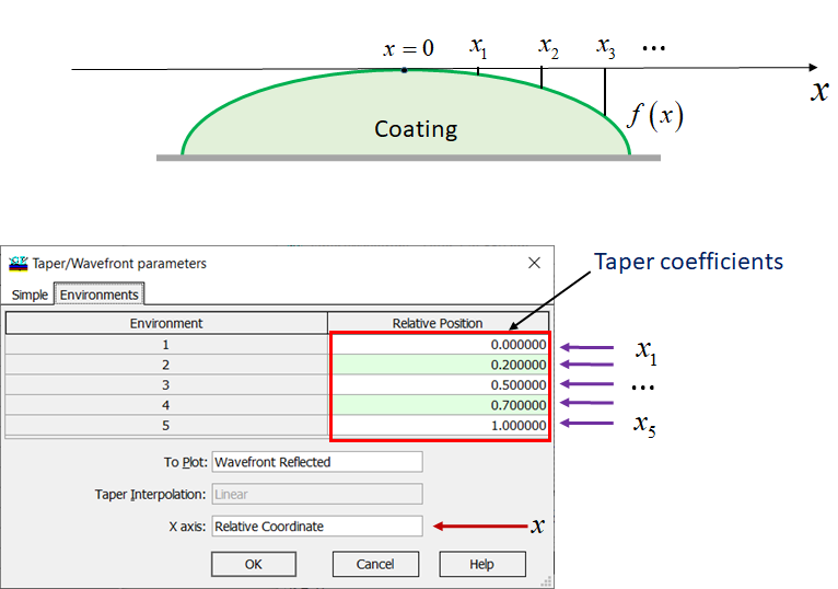
Fig. 7. Specification of taper coefficients in the environment manager. |
Reflected/transmitted wavefront can be calculated for more complicated taper interpolations specified through Taper coefficients in the Environments manager (Data –> Environments manager) (Fig. 7) and Relative Positions (Fig. 8).
Fig. 8. Schematic of a complicated taper interpolation and the correspondence window in OptiLayer. |
|
OptiLayer allows you to calculate dependence of spectral characteristics (reflectance, transmittance, phase, GD, and GDD) on the relatvive coordinate and on the wavlength. Fig. 9. Schematic of a coating with layer non-uniformity. |
Fig. 10. Schematic of the coating with layer non-uniformity at central position (left) and at position \(x_1\) (right). Computations of spectral characteristics (reflectance, transmittance, phase, GD, and GDD) are performed at each relative coordinate/wavelength using standard formulas. |
|
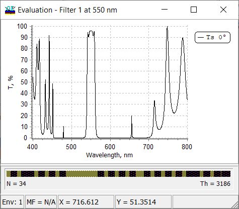
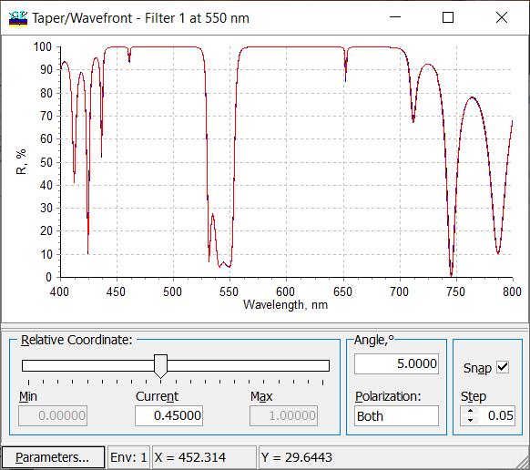
Fig. 11. Wavelength dependence of reflectance at a relative coordinate of 0.45. You can vary the relative position using the slider. Also, you can vary the angle of incidence and polarization (s, p or average (both)). |
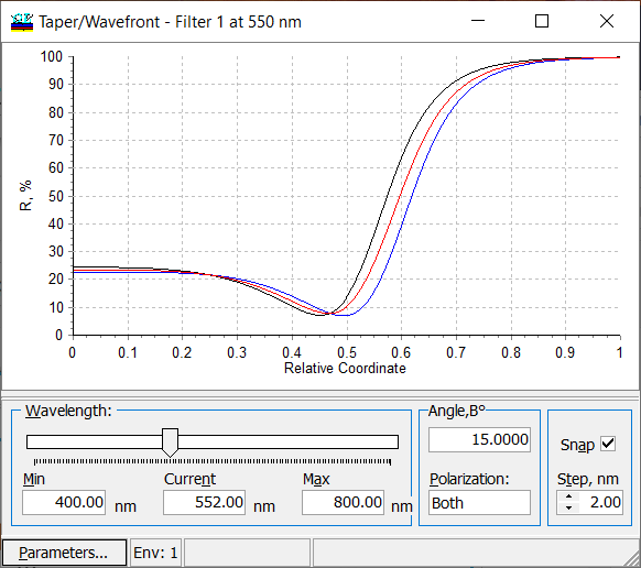
Fig. 12. Dependence of the coating reflectance on the position at the wavelength of 552nm. You can vary the wavelength with the help of the slider. Also, you can vary the angle of incidence and polarization (s, p or average (both)). |
OptiLayer provides user-friendly interface and a variety of examples allowing even a beginner to effectively start to design and characterize optical coatings. Read more…
Comprehensive manual in PDF format and e-mail support help you at each step of your work with OptiLayer.
If you are already an experienced user, OptiLayer gives your almost unlimited opportunities in solving all problems arising in design-production chain. Visit our publications page.
Look our video examples at YouTube
OptiLayer videos are available here:
Overview of Design/Analysis options of OptiLayer and overview of Characterization/Reverse Engineering options.
The videos were presented at the joint Agilent/OptiLayer webinar.